ds_journal - Entity Embedding in fastai 2

This post aims to introduce how to use fastai v2 to implement entity embedding for categorical variables in tabular data. Entity embedding is a powerful technique that can sometimes boost the performance of various machine learning methods and reveal the intrinsic properties of categorical variables. See this paper and this post for more details.

import seaborn as sns
from fastai.tabular.all import *

Get Data

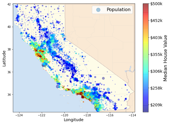
We will use the California housing dataset for this post. We want to develop a model to predict the median_house_value based on other variables in the dataset. The following code shows the first 5 rows of the dataset.

df = pd.read_csv('housing.csv')
df.head()

	longitude	latitude	housing_median_age	total_rooms	total_bedrooms	population	households	median_income	median_house_value	ocean_proximity
0	-122.23	37.88	41.0	880.0	129.0	322.0	126.0	8.3252	452600.0	NEAR BAY
1	-122.22	37.86	21.0	7099.0	1106.0	2401.0	1138.0	8.3014	358500.0	NEAR BAY
2	-122.24	37.85	52.0	1467.0	190.0	496.0	177.0	7.2574	352100.0	NEAR BAY
3	-122.25	37.85	52.0	1274.0	235.0	558.0	219.0	5.6431	341300.0	NEAR BAY
4	-122.25	37.85	52.0	1627.0	280.0	565.0	259.0	3.8462	342200.0	NEAR BAY

Preprocess Data

We rely on various functionalities provided by fastai to preprocess the data. We will not discuss them in detail here. For more information, please check this tutorial. One important note is that when dealing with categorical variables, instead of using one-hot encoding, we map each category into a distinct integer.

cont, cat = cont_cat_split(df, dep_var = 'median_house_value')

splits = RandomSplitter(valid_pct=0.2)(range_of(df))

to = TabularPandas(df, procs=[Categorify, FillMissing,Normalize],
                   cat_names = cat,
                   cont_names = cont,
                   y_names='median_house_value',
                   splits=splits)

dls = to.dataloaders(bs=64)

Train Model

We will train a deep learning model to predict the median housing value and thus get the trained embedding for categorical variables. Again, see this tutorial for details about the meaning of the codes here.

learn = tabular_learner(dls, metrics=rmse)

early_stop_cb = EarlyStoppingCallback(patience=2)

#collapse-output
learn.fit_one_cycle(10, cbs=early_stop_cb)

epoch	train_loss	valid_loss	_rmse	time
0	55994937344.000000	56636186624.000000	237983.578125	00:04
1	56567816192.000000	56058937344.000000	236767.671875	00:04
2	52564221952.000000	52214001664.000000	228503.843750	00:03
3	45972250624.000000	46276349952.000000	215119.375000	00:03
4	37385846784.000000	37008117760.000000	192374.937500	00:03
5	31154010112.000000	30351321088.000000	174216.312500	00:03
6	24364992512.000000	23757260800.000000	154133.906250	00:03
7	22229555200.000000	21549965312.000000	146799.031250	00:03
8	20496922624.000000	21110308864.000000	145293.875000	00:03
9	20571899904.000000	20511488000.000000	143218.312500	00:03

Get Embedding

We will retrieve the trained embedding matrix from the model.

embs = [param for param in learn.model.embeds.parameters()]

The list has two elements and each element represents an embedding matrix for a categorical variable.

len(embs)

To check what each element corresponds to, we can use the cat_names attributes from TabularPandas. The list indicates that the first element in embs is the embedding matrix for the variable ocean_proximity.

to.cat_names

(#2) ['ocean_proximity','total_bedrooms_na']

Let’s see this matrix. Note that we convert it from a tensor array to a numpy array to make the operation later easier.

ocean_emb = embs[0].detach().numpy()
ocean_emb

array([[ 0.00074246,  0.01322438, -0.00539126,  0.00066858],
       [-0.01550745, -0.02467075,  0.01956671, -0.01148492],
       [ 0.24266721,  0.35117084, -0.35875005,  0.36369336],
       [-0.05629548, -0.06088502,  0.08677642, -0.10355063],
       [-0.01115109, -0.02015582,  0.01277605, -0.00476734],
       [-0.01796132, -0.02396758,  0.02242134, -0.0143294 ]],
      dtype=float32)

Each row in the matrix above corresponds to one category in the categorical variable. The categories for ocean_proximity are the following.

cat = to.procs.categorify
ocean_cat = cat['ocean_proximity']
ocean_cat

['#na#', '<1H OCEAN', 'INLAND', 'ISLAND', 'NEAR BAY', 'NEAR OCEAN']

We can use the o2i attribute to see how each category is mapped into an integer. The integer corresponds to the row in the embedding matrix.

ocean_cat.o2i

defaultdict(int,
            {'#na#': 0,
             '<1H OCEAN': 1,
             'INLAND': 2,
             'ISLAND': 3,
             'NEAR BAY': 4,
             'NEAR OCEAN': 5})

For example, the embedding for ‘NEAR BAY’ is:

ocean_emb[4]

array([-0.01115109, -0.02015582,  0.01277605, -0.00476734], dtype=float32)

Let’s create a dictionary to map each category to its corresponding embedding.

ocean_emb_map = {ocean_cat[i]:ocean_emb[i] for i in range(len(ocean_cat))}

Apply Embedding

This section shows how we can apply the embedding to the original dataset; that is, change the category variable to numeric vectors.

emb_dim = ocean_emb.shape[1]

col_name = [f'ocean_emb_{i}' for i in range(1,emb_dim+1)]
df_emb = pd.DataFrame(df['ocean_proximity'].map(ocean_emb_map).to_list(), columns=col_name)
df_emb.head()

	ocean_emb_1	ocean_emb_2	ocean_emb_3	ocean_emb_4
0	-0.011151	-0.020156	0.012776	-0.004767
1	-0.011151	-0.020156	0.012776	-0.004767
2	-0.011151	-0.020156	0.012776	-0.004767
3	-0.011151	-0.020156	0.012776	-0.004767
4	-0.011151	-0.020156	0.012776	-0.004767

df_new = pd.concat([df, df_emb],axis=1)

Visualize Embedding

Another way to explore the embedding matrix is to visualize it and see what it learns. We will use principle component analysis(PCA) to visualize the embedding.

from sklearn import decomposition
pca = decomposition.PCA(n_components=2)
pca_result = pca.fit_transform(ocean_emb)

df_visualize = pd.DataFrame({'name':ocean_cat, 'dim1':pca_result[:,0], 'dim2':
                             pca_result[:,1]})
sns.scatterplot(data=df_visualize, x='dim1', y='dim2', hue='name');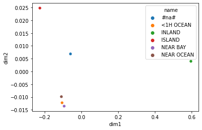

If we compare this visualization to the map of these houses above, we will find that the embedding matrix does provide some useful insights. In particular, we see that the relative location of the category INLAND does correspond to the inland area in the map. The code to make the following map comes from this notebook.

Ending Note

This is the end of this post. You can see the full code by clicking to the View on Github or Open in Colab tab at the top this post.